Relations between some linear decoding and LPN algorithms

Introduction

This note describes some connections between algorithms for decoding linear codes and for solving LPN problems. They are quite simple but many lectures on decoding skip them, so I decided to write it down.

Let's start with definitions.

LPN problem: given a matrix $A \in \F^{n\times k}$, $k < n$, a vector $\vec{b} \in \F^n$ and an error rate $\tau \in [0,1/2)$, find $\vec{x} \in \F^k$ such that $\vec{e} = \wt(\vec{b}-A\vec{x}) \le \tau n$. Note: usually, LPN allows an arbitrary number of random queries, in this note I'll stick to a fixed number $n$.

Syndrome decoding: given a parity check matrix $H \in \F^{m\times n}$, $m < n$, a syndrome $\vec{s} \in \F^m$ and the number of errors $t$, find $\vec{e} \in \F^n$ such that $H \vec{e} = \vec{s}$ and $\wt(\vec{e}) \le t$.

The LPN problem can be interpreted as solving a system of linear equations minimizing errors, while syndrome decoding is about finding a "short" but exact solution (short in the Hamming weight metric). Although LPN traditionally implies the binary field ($\F = \F_2$), all these ideas apply to any field.

By transposing the LPN problem $A\vec{x} + \vec{e} = \vec{b}$ into $\vec{x} G + \vec{e} = \vec{b}$ with $G = A^T$, we get a usual notation for the problem of decoding a linear code with the generator matrix $G = A^T$, for which syndrome decoding is an equivalent (dual) formulation. This post explores this connection with relation to decoding algorithms in the two formulations.

Prange vs PooledGauss

There is a basic algorithm for each of the two problems.

• PooledGauss: For LPN, the algorithm is considered folklore and was called PooledGauss and analyzed in details in [EKM17]. The idea is to randomly select $k$ (out of $n$) independent equations (rows of $A$), hoping that these equations have no errors in the target solution. The equations can be sampled from a small prepared set of equations (the "pool"). Solving the corresponding system $A\vert_I \vec{x} = \vec{b}\vert_I$, where $I$ denotes the chosen rows, yields a full candidate $\vec{x}$ for which it only remains to test the number of errors on the full system $A \vec{x} = \vec{b}$.
• Prange: For syndrome decoding, the classic algorithm is due to Prange [Pra62]. The idea is to randomly select $m$ (out of $n$) columns of $H$, hoping that the target solution's columns fall inside the selection. Then, solving $H\vert^{J} \vec{e}\vert^{J} = \vec{s}$ yields a candidate solution $\vec{e}$ (by filling $\vec{e}\vert^{J}$ with zeroes), the weight of which can be checked directly (here $J$ denotes the selected columns).
  Remark on Prange's method: often in lectures Prange's algorithm is presented as inverting the selected columns $Q=(H\vert^{J})^{-1}$ and computing $\vec{e}\vert^J=Q\vec{s}$. But solving directly (instead of matrix inversion and multiplication) can be faster in practice by a small factor. On the other hand, inversion-based approach is more useful for further optimizations and can be amortized, so it's not important in the end.

These two problems and algorithms are in fact almost the same things, and can be viewed as duals of each other. To see that, let's rephrase the LPN problem in terms of usual linear code notation. Let $G = A^{T}$. Then,

$A \vec{x} + \vec{e}= \vec{x} G + \vec{e}= \vec{b},$

which is clearly the problem of decoding a corrupted codeword $\vec{b}$ from the linear $[n,k]$-code with the generator matrix $G \in \F^{k \times n}$. Now, a corresponding parity check matrix $H$ is determined by $H^TG = 0$, so that $H \times (\vec{x}G)^T = 0$ for all $\vec{x}$. It has dimensions $(n-k) \times n$. Let $\vec{s} = H \times \vec{b} = H \times (A\vec{x} + \vec{e}) = H \vec{e}$ be the syndrome. Note that we can compute $\vec{s}$ since we know $H$ and $\vec{b}$. As a result, we converted the original (pooled) LPN problem $A \vec{x} + \vec{e} = \vec{x} G + \vec{e} = \vec{b}$ (low-weight $\vec{e}$) into syndrome decoding $H \vec{e} = \vec{s}$ (low-weight $\vec{e}$).

To see the connection between the two algorithms, it is convenient to stack $G=A^T$ over $H$ to form a square $n\times n$ matrix:

Figure: Generator matrix and parity check matrix of a linear code

Then, it becomes clear that a choice $I$ of rows of $A$ (columns of $G$) in the PooledGauss algorithm is in fact complementary to the choice $J$ of columns of $H$ in the Prange's algorithm:

Figure: Relation between square submatrices selected in PooledGauss and Prange's method

In this picture, the "*" symbols denote potential nonzero entries of the error vector $\vec{e}$. The PooledGauss algorithm suceeds when all the errors are outside of the chosen invertible equation matrix $G\vert^I$, while Prange's algorithm succeeds when all the errors are inside the chosen invertible parity check submatrix $H\vert^J$. Clearly, such successful choices are in bijection by $J=\overline{I}$.

This also shows that PooledGauss is faster than Prange's algorithm whenever $G$ is long ($k < n-k$, as in the figure), and vice versa, because the respective matrix inversion steps cost $k^3$ and $(n-k)^3$ respectively. Again, better algorithms amortize the inversion costs and it becomes irrelevant.

Blum-Kalai-Wasserman (BKW) vs Wagner's generalized birthday

Another closely related methods are BKW [BKW00] and Wagner's generalized birthday / $k$-sum algorithm [Wag02].

BKW algorithm for LPN

Similarly to the previous algorithms, the idea of BKW departs from the Gaussian elimination. But now, instead of starting with $k$ potentially error-free samples, we will use more samples and allow errors in them. The idea is to add as few samples together as possible to arrive at a chosen weight-1 sample. The resulting equation would be of the form $x_i = c + e'$ where $c$ is a constant and $e'$ is a combined error (equal to to the sum of errors of the added sampleds). The combined error will be worse than the original one, but now we essentially have a 1-variable LPN instance. After collecting enough such equations for the same variable $x_i$ we can learn it by taking the most frequent value $c$. The number of samples is polynomial in $|1/2-\tau'|$, where $\tau'$ is the probability of $e'=1$.

How do we perform Gaussian elimination with small number of additions? The idea of BKW is to simply perform block-wise elimination: instead of eliminating 1 variable at a time, we can eliminate $B$ variables at time given that we have many collisions in values of these $B$ variables (meaning that we need quite more than $2^B$ samples). Then, each reduced vector would only take $\lceil n/B \rceil$ additions to make.

Remark: the large sample requirement means that BKW is only applicable to decoding $[n,k]$-codes with large $n/k$ ratio. However, one can "inflate" the code by randomly adding pairs of samples, at the cost of increasing the error probability.

Remark: the last row addition can be saved by not reducing the last block and using fast Walsh-Hadamard transform (FWHT) to recover the solution in time $\mathcal{O}(B2^B)$.

Wagner's $k$-sum problem

Wagner considered the following problem as a generalization of the birthday paradox.

$k$-sum problem. Given lists $L_1,\ldots,L_k \subseteq \F_2^n$, find $x_1\in L_1, \ldots, x_k \in L_k$ such that $x_1 \oplus x_2 \oplus \ldots \oplus x_k = 0$.

Wagner proposes the following recursive approach (called $k$-tree algorithm) to solve this problem. Merge lists in pairs $(L_1,L_2),(L_3,L_4),\ldots$ by adding all possible pairs of elements from the two lists and filtering them in the first $\ell$ bits: $$L'_i = L_{2i} \bowtie L_{2i+1} = \{x \oplus x' \mid x \in L_{2i}, x' \in L_{2i+1}, (x \oplus x')_{1,...\ell} = 0\}.$$ Then, repeat the procedure on the resulting lists to match $2\ell$ bits, $3\ell$ bits, etc. For a correct relation between $k$ and $\ell$, this would result in a solution to the problem.

The resulting structure of list merges form a binary tree.

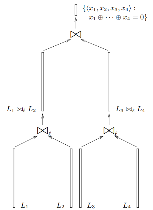
Figure: Wagner's $k$-sum algorithm (credits: [Wag02])

Extension 1: it is easy to see that solving $x_1 \oplus x_2 \oplus \ldots \oplus x_k = c$ for any chosen constant vector $c \in \F_2^n$ is not harder: simply replace the list $L_1$ with $L_1 \oplus c$ and solve the zero-sum problem for lists $L_1 \oplus c, L_2, \ldots, L_k$.

Extension 2: often in applications all the lists are the same ($L_1 = L_2 = \ldots = L_k = L$). Here, the zero-sum problem becomes trovial when $k$ is even. But the case of non-zero target is still similarly hard as the original problem. Furthermore, it allows an optimization of the algorithm: instead of the tree-like structure depicted above, the zero-sum

Although not usually stated as such, the $k$-sum problem (more precisely, the two extensions/simplifications described above) can be viewed as the syndrome decoding problem: the list $L$ corresponds to the columns of the parity check matrix $H$, and we aim to find a weight-$k$ vector $\vec{e}$ such that $H \vec{e} = \vec{s}$. However, the $k$-tree algorithm targets the "dense" case, where the number of solutions is very large and it is sufficient to get any of them, while most decoding problems only have a unique solution. Therefore, the $k$-tree algorithm is often not directly applicable, but is still used as a subprocedure in more advanced decoding algorithms.

The relation

It may be difficult to see that the first part of the BKW algorithm and the $k$-tree algorithm are equivalent. The problem is that (block-wise) Gaussian elimination seems iterative in nature and hides the tree-like structure of additions. However, careful observation shows that the BKW algorithm simply performs the $k$-tree algorithm with $L$ being the rows of the equation matrix $A$ and the target vector being a chosen unit vector, e.g. $(1,0,\ldots,0)$.

Note that Wagner writes that BKW is closely related to his $k$-tree algorithm in [Wag02].